An R Package for Causal Effect Estimation via the Front-Door Functional
This R package implements methods for estimating the average treatment effect (ATE) and the average treatment effect on under the front-door model (Pearl, 1995). The implementation follows the estimators proposed in Guo et al. (2023), based on influence function theory and targeted minimum loss-based estimation (TMLE).
If you find this package useful, please cite:
@article{guo2023flexible,
  title={Flexible nonparametric inference for causal effects under the front-door model},
  author={Guo, Anna and Benkeser, David and Nabi, Razieh},
  journal={arXiv preprint arXiv:2312.10234},
  year={2023}
}
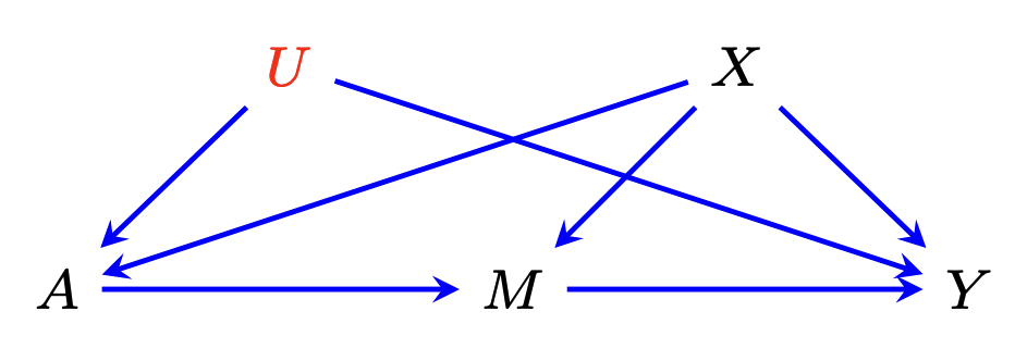
The front-door setting involves:
-
A: treatment (binary) -
M: mediator(s) -
Y: outcome -
X: observed confounder(s) -
U: unobserved confounder(s)
This package supports estimation of both the Average Treatment Effect (ATE) and the Average Treatment Effect on the Treated (ATT) under a binary treatment. In the discussion of nuisance estimation below, we focus on ATE estimation. The same principles and procedures apply to ATT estimation.
For ease of exposition, we consider the average counterfactual outcome under treatment level (A = a_0), denoted by (E(Y^{a_0})), as the target parameter of interest. The ATE can therefore be expressed as (E(Y^1) - E(Y^0)).
Under the front-door model, the parameter (E(Y^{a_0})) is identified through the following identification (ID) functional, where (P) denotes the true observed data distribution:
\[\begin{align*} \psi(P) = \iint \sum_{a=0}^1 y \ p(y \mid m, a, x) \ p(a \mid x) \ p(m \mid A=a_0, x) \ p(x) \ dy \ dm\ dx \ . \quad \text{(target parameter)} \end{align*}\]For a detailed description of the proposed estimators for this estimand, see [Guo et al. 2023]. The remainder of this document describes the installation of the package and the use of its main function.
1. How to Use
Installation
To install the package from GitHub:
install.packages("remotes") # If you have not installed "remotes" package
remotes::install_github("annaguo-bios/fdcausal")
The source code for fdcausal package is available on GitHub at fdcausal.
Description
The fdcausal package provides the function estfd(), which implements both one-step estimators and TMLEs for both ATE and ATT.
The package includes several example datasets, inclduing continuousY_continuousM, continuousY_continuousM_10dX, and binaryY_binaryM, which are used throughout this tutorial to demonstrate the usage of estfd(). Details of the corresponding data-generating processes (DGPs) are provided in Section 4.
An example of calling estfd() with a minimal set of arguments is shown below. This example estimates the ATE using the one-step estimator under the default nuisance estimation methods:
cYcM_ATE <- estfd(a=c(1,0), data=continuousY_continuousM,
             treatment="A", mediators="M", outcome="Y", covariates="X",
             estimator='onestep')
To estimate ATT, add ATT = T
cYcM_ATT <- estfd(a=c(1,0), data=continuousY_continuousM,
             treatment="A", mediators="M", outcome="Y", covariates="X",
             estimator='onestep', ATT = T)
The estfd() function includes additional arguments that primarily control how the nuisance functions are estimated. A brief discussion of nuisance estimation is provided in the following section.
2. Detailed Discussion on Implementation
The front-door identification functional involves four nuisance functionals: the outcome regression (E(Y \mid M, A, X)), the propensity score (p(A \mid X)), the mediator density (p(M \mid A, X)), and the marginal distribution of the measured confounder(s) (p(X)). Let (Q) denote this collection: (Q = {E(Y \mid M, A, X), p(A \mid X), p(M \mid A, X), p(X)}). The package provides multiple approaches for estimating these nuisance functionals, as described below.
2.1 Nuisance estimation
- [Regression]{style=”color:red;”}: The default approach for estimating (E(Y \mid M, A, X)) and (p(A \mid X)) uses linear or logistic regression. When the mediator is univariate and binary, the mediator density (f_M(M \mid A, X)) is also estimated using logistic regression. For other types of mediators, alternative approaches are discussed in the next subsection. When regression-based methods are used, the package allows users to specify model formulas via the arguments
formulaY,formulaA, andformulaM, corresponding to the outcome regression, propensity score, and mediator density, respectively. For binary variables, the link function in logistic regression can be specified usinglinkY_binary,linkA, andlinkM_binary.
For example:
  bYbM <- estfd(a=1,data=binaryY_binaryM,
               treatment="A", mediators="M", outcome="Y", covariates="X",
               estimator='onestep',
               formulaY="Y ~ .", formulaA="A ~ .", formulaM="M~.",
               linkY_binary="logit", linkA="identity", linkM_binary="logit")
where a=1 returns estimation results for (E(Y^1)).
-
Super Learner: use argument
superlearner=Tin theestfd()function to estimate nuisance functionals with the SuperLearner package. The SuperLearner is an ensemble algorithm that combines estimates from various statistical and machine learning models, creating a more adaptable and robust estimation scheme. The default algorithms used for superlearner in the fdcausal package arec("SL.glm","SL.earth","SL.ranger","SL.mean"). Users, however, can specify any algorithms incorporated in the SuperLearner package. -
Cross-fitting with Super Learner: use the
crossfit=Targument in theestfd()function to estimate nuisance functionals using cross-fitting in conjunction with the use of a super learner. The number of folds can be adjusted using the argumentKwith the default being set to (K=5). As an example, the following code runs ATE estimation using random forest combined with cross-fitting of (2) folds.
cYcM <- estfd(a=c(1,0), data=continuousY_continuousM_10dX,
             treatment="A", mediators="M", outcome="Y", covariates=paste0("X.",1:10),
             estimator='onestep', crossfit=T, lib = c("SL.ranger"), K=2)
2.2 Estimation under different types of mediators
This package incorporates different estimation schemes tailored to various types of mediators. As mentioned above, (f_M(M\mid A,X)) is estimated via logistic regression under a binary mediator (M). Different estimation strategies would be needed to handle other types of mediators, due to the complexity of (conditional) density estimations. We offer four different options to deal with the complexity of mediator density estimation. The choice can be controlled by argument mediator.method.
-
mediator.method=np: This method corresponds to direct estimation and targeting of the mediator density. Whennp.dnorm=F, (f_M(M\mid A,X)) is estimated using the nonparametric kernel method via the np package. Whennp.dnorm=T, (f_M(M\mid A,X)) is estimated assuming normal distribution. The mean of the normal distribution is estimated via the regression of (M) on (A) and (X), and the standard deviation of the normal distribution is estimated via the sample standard devation of the error term in the regression. Given the computational burden imposed by direct estimation of the mediator density, thisnpmethod is only applicable to univariate continuous mediator. -
mediator.method=densratio: This method circumvents direct estimation of the mediator density by estimating its ratio (f_M(M\mid A=a_0,X)/f_M(M\mid A,X)) instead, where (a_0) is the treatment assignment of interest. For the density ratio estimation we use the densratio package. -
\[\frac{f_M(M\mid A=a,X)}{f_M(M\mid A,X)} = \frac{p(a_0 \mid X, M)}{p(A \mid X, M)} \times \frac{\pi(A \mid X)}{\pi(a_0 \mid X)}.\]mediator.method=bayes: This method estimates density ratio (f_M(M\mid A=a,X)/f_M(M\mid A,X)) by reformulating it using the Bayes’ rule as follows:The density ratio is estimated via estimating (p(A \mid X, M)) and (\pi(A\mid X)). (p(A \mid X, M)) can be estimated via super learner, cross-fitting in conjunction with super learner, or logistic regression. When using logistic regression,
formula_bayesandlink_bayesarguments inestfd()allow users to specify the formula and link function used in the logistic regression. -
mediator.method=dnorm: This method estimates density ratio, assuming that (M\mid A,X) follows conditional normal distribution. The mean and standard deviation of the normal distribution are estimated using the same strategy as discussed in themediator.method=nppart. Estimates of the density ratio is then constructed as the ratio of the density estimates. Summary: Thenpmethod allows estimation under univariate continuous mediator, while thedensratio, bayes, dnormmethods work for both univariate and multivariate mediators. The mediators can be binary, continuous, or a mix. Thenpmethod involves direct estimation of the mediator density, and the targeting step of the TMLE would require iterative updates between the outcome regression, propensity score, and mediator density. Consequently, this method is computationally more intensive. The TMLE procedure underdensratio, bayes, dnormdoes not require iterative updates among the nuisance functionals. Therefore, those methods are more computationally efficient and are especially appealing in settings with multivariate mediators.
3. Output
The output of the estfd() function depends on the mediator.method used. As an example, we use mediator.method=np to estimate the average counterfactual outcome (E(Y^1)). The output is described as follows
# Set a=1 returns estimation results on E(Y)
cYcM <- estfd(a=1, data=continuousY_continuousM,
             treatment="A", mediators="M", outcome="Y", covariates="X",
             estimator=c('onestep','tmle'), mediator.method="np")

## TMLE output ##
cYcM$TMLE$estimated_psi # point estimate of the target parameter E(Y^1).
cYcM$TMLE$lower.ci # lower bound of the 95% confidence interval for the E(Y^1) estimate.
cYcM$TMLE$upper.ci # upper bound of the 95% confidence interval for the E(Y^1) estimate.
cYcM$TMLE$p.M.aX # mediator density estimate at treatment level A=a.
cYcM$TMLE$p.M.AX # mediator density estimate at treatment level A=A.
cYcM$TMLE$p.a1.X_updated # propensity score estimate at treatment level A=1.
cYcM$TMLE$or_pred_updated # outcome regression estimate.
cYcM$TMLE$EIF # estimated efficient influence function evaluated at all observations.
              #EIF can be used to construct confidence interval for E(Y^1).
cYcM$TMLE$EDstar # a vector composes of the sample average of the projection of EIF onto the tangent space corresponding to Y|M,A,X; M|A,X; and A|X.
                 # upon convergence of the algorithm, elements of this vector should be close to 0.
cYcM$TMLE$EDstar_M.vec # sample average of the projection of EIF onto tangent space of M|A,X over iterative updates of the nuisance functionals.
                       # the elements in this vector should converge to zero over iterations.
cYcM$TMLE$EDstar_ps.vec # sample average of the projection of EIF onto tangent space of A|X over iterative updates of the nuisance functionals.
                        # the elements in this vector should converge to zero over iterations.
cYcM$TMLE$eps2_vec # the indexing parameter for submodels for the mediator density over iterations.
                   # the elements in this vector should converge to zero over iterations.
cYcM$TMLE$eps3_vec # the indexing parameter for submodels for the propensity score over iterations.
                   # the elements in this vector should converge to zero over iterations.
cYcM$TMLE$iter # number of iterations upon convergence.

## One-step estimator output ##
cYcM$Onestep$estimated_psi # point estimate of the target parameter E(Y^1).
cYcM$Onestep$theta_x # estimate of theta(X) as defined in the Section~3
cYcM$Onestep$lower.ci # lower bound of the 95% confidence interval for the E(Y^1) estimate.
cYcM$Onestep$upper.ci # upper bound of the 95% confidence interval for the E(Y^1) estimate.
cYcM$Onestep$EIF # estimated efficient influence function evaluated at all observations.
cYcM$Onestep$EDstar # a vector composes of the sample average of the projection of EIF onto the tangent space corresponding to Y|M,A,X; M|A,X; and A|X.
In the following, we use mediator.method=bayes to estimate ATE. The output is described as follows
cYcM <- estfd(a=c(1,0), data=continuousY_continuousM_10dX,
             treatment="A", mediators="M", outcome="Y", covariates=paste0("X.",1:10),
             onestep=T, mediator.method = "bayes")

## TMLE output ##
ATE <- cYcM$TMLE$ATE # point estimate of the target parameter ATE.
lower.ci <- cYcM$TMLE$lower.ci # lower bound of the 95% confidence interval for the ATE estimate.
upper.ci <- cYcM$TMLE$upper.ci # upper bound of the 95% confidence interval for the ATE estimate.
EIF <- cYcM$TMLE$EIF # estimated efficient influence function evaluated at all observations.
                     #EIF can be used to construct confidence interval for E(Y^1).

E.Y1.obj <- cYcM$TMLE.Y1 # oject containing estimation results on E(Y^1).
E.Y1.obj$estimated_psi # point estimate of the target parameter E(Y^1).
E.Y1.obj$lower.ci # lower bound of the 95% confidence interval for the E(Y^1) estimate.
E.Y1.obj$upper.ci # upper bound of the 95% confidence interval for the E(Y^1) estimate.
E.Y1.obj$theta_x # estimate of theta(X) as defined in the Section~3
E.Y1.obj$M.AXratio # estimate of the mediator density ratio f_M(M|A=1,X)/f_M(M|A,X)
E.Y1.obj$p.a1.X # propensity score estimate at treatment level A=1.
E.Y1.obj$or_pred # outcome regression estimate.
E.Y1.obj$EIF # estimated efficient influence function evaluated at all observations.
              #EIF can be used to construct confidence interval for E(Y^1).
E.Y1.obj$EDstar # estimated efficient influence function evaluated at all observations.
              #EIF can be used to construct confidence interval for E(Y^1).


E.Y0.obj <- cYcM$TMLE.Y0 # oject containing estimation results on E(Y^0)
# similar story as E.Y1.obj#

## One-step estimator output ##
ATE <- cYcM$Onestep$ATE # point estimate of the target parameter ATE.
lower.ci <- cYcM$Onestep$lower.ci # lower bound of the 95% confidence interval for the ATE estimate.
upper.ci <- cYcM$Onestep$upper.ci # upper bound of the 95% confidence interval for the ATE estimate.
EIF <- cYcM$Onestep$EIF # estimated efficient influence function evaluated at all observations.
              #EIF can be used to construct confidence interval for E(Y^1).

E.Y1.obj <- cYcM$Onestep.Y1
# similar story as E.Y1.obj for TMLE #

E.Y0.obj <- cYcM$Onestep.Y0
# similar story as E.Y1.obj for TMLE #
Outputs under mediator methods densratio, dnorm are the same as above.
4 Illustrative DGPs
Here, we briefly look at the continuousY_continuousM dataset.
str(continuousY_continuousM)
'data.frame':   500 obs. of  5 variables:
 $ X: num  0.467 0.338 0.686 0.755 0.137 ...
 $ U: num  3.0707 2.0449 2.521 3.591 0.0665 ...
 $ A: int  1 0 0 1 0 1 0 0 1 0 ...
 $ M: num  2.095 0.527 2.569 4.022 3.189 ...
 $ Y: num  6.22 3.19 5.47 9.45 2.82 ...
This dataset is generated with the following DGP
set.seed(7)

## generate continuous outcome Y, continuous mediator M, single measured covariate X====
generate_data <- function(n,parA = c(0.3,0.2), parU=c(1,1,1,0), parM = c(1,1,1,0), parY = c(1, 1, 1, 0), sd.M=1, sd.U=1, sd.Y=1){

  X <- runif(n, 0, 1) # p(X)

  A <- rbinom(n, 1, (parA[1] + parA[2]*X)) # p(A|X)

  U <- parU[1] + parU[2]*A + parU[3]*X + parU[4]*A*X + rnorm(n,0,sd.U) # p(U|A,X)

  M <- parM[1] + parM[2]*A + parM[3]*X + parM[4]*A*X + rnorm(n,0,sd.M) # p(M|A,X)

  Y <- parY[1]*U + parY[2]*M + parY[3]*X + parY[4]*M*X + rnorm(n, 0, sd.Y) # p(Y|U,M,X)

  data <- data.frame(X=X, U=U, A=A, M=M, Y=Y)

  # propensity score
  ps <- A*(parA[1] + parA[2]*X)+(1-A)*(1-(parA[1] + parA[2]*X))

  # mediator density ratio: p(M|a,X)/p(M|A,X)
  m.ratio.a1 <- dnorm(M,parM[1] + parM[2]*1 + parM[3]*X + parM[4]*1*X,sd.M)/dnorm(M,parM[1] + parM[2]*A + parM[3]*X + parM[4]*A*X,sd.M)
  m.ratio.a0 <- dnorm(M,parM[1] + parM[2]*0 + parM[3]*X + parM[4]*0*X,sd.M)/dnorm(M,parM[1] + parM[2]*A + parM[3]*X + parM[4]*A*X,sd.M)

  return(list(data = data,
              parA=parA,
              parU=parU,
              parM=parM,
              parY=parY,
              sd.U=sd.U,
              sd.Y=sd.Y,
              sd.M=sd.M,
              ps=ps,
              m.ratio.a1=m.ratio.a1,
              m.ratio.a0=m.ratio.a0))
}

continuousY_continuousM <- generate_data(500)$data
References
- [Guo et al. 2023] Guo, A., Benkeser, D., & Nabi, R. Flexible nonparametric inference for causal effects under the front-door model. arXiv preprint arXiv:2312.10234, 2023.
- [Pearl. 1995] Pearl, J. Causal diagrams for empirical research. Biometrika, 1995.
- [Fulcher et al. 2019] Fulcher I R, Shpitser I, Marealle S, & Tchetgen Tchetgen, E. Robust inference on population indirect causal effects: the generalized front door criterion. Royal Statistical Society Series B: Statistical Methodology, 2020.
- [Van der Laan et al. 2011] Van der Laan M J, Rose S. Targeted learning: causal inference for observational and experimental data. New York: Springer, 2011.