An R Package for Causal Effect Estimation in the Napkin Graph
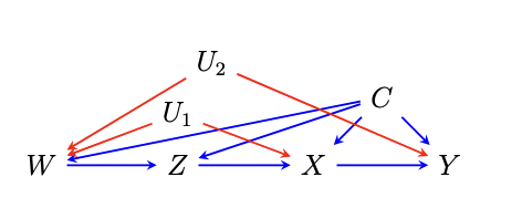
This package is built for estimating the Average Causal Effect (ACE) in the Napkin graphical model. This package is an implementation of the proposed estimators by Guo et al., 2025, based on the theory of influence functions and targeted minimum loss based estimation (TMLE).
If you find this package useful, please cite:
@article{guo2025causal,
  title={Causal Inference with the Napkin Graph},
  author={Guo, Anna and Liu, Lin and Benkeser, David and Nabi, Razieh},
  journal={arXiv preprint arXiv:2512.19861},
  year={2025}
}
Overview
napkincausal estimates average counterfactual outcomes and average causal effects in the Napkin graph. The main user-facing function is napkin_est(), which returns targeted minimum loss-based estimators (TMLE), one-step estimators, and, when applicable, estimating-equation estimators.
The package supports binary or continuous outcomes, binary or continuous Z, user-specified intervention densities for continuous Z, SuperLearner nuisance estimation, and optional cross-fitting. When baseline covariates are supplied through covariates, napkin_est() uses the covariate-adjusted estimator.
Installation
You can install the development version from a local copy of the package:
install.packages("remotes") # If you have not installed "remotes" package
remotes::install_github("annaguo-bios/napkincausal")
Then load the package:
library(napkincausal)
Basic Usage
The core arguments are:
-
x: treatment level, orc(1, 0)for an average causal effect. -
data: a data frame containing the observed variables. -
treatment: treatment variable name. -
Z.variables: mediator/intervention variable name. -
W.variables: parent variable name forZ. -
outcome: outcome variable name.
For example, to estimate E(Y(1)) using one of the included example datasets:
data(data_Zbinary_Ycontinuous)

fit <- napkin_est(
  x = 1,
  data = data_Zbinary_Ycontinuous,
  treatment = "X",
  Z.variables = "Z",
  W.variables = "W",
  outcome = "Y",
  formula.Y = "Y ~ .",
  formula.X = "X ~ .",
  formula.Z = "Z ~ .",
  verbose = FALSE
)
## Onestep estimated E(Y(1)) for z=1: 5.57;95% CI: (5.49,5.66)
## Onestep estimated E(Y(1)) for z=0: 5.51;95% CI: (5.43,5.59)
## Onestep estimated E(Y(1)) for z=all z: 5.54;95% CI: (5.48,5.61)
## TMLE estimated E(Y(1)) for z=1: 5.58;95% CI: (5.5,5.67)
## TMLE estimated E(Y(1)) for z=0: 5.51;95% CI: (5.42,5.59)
## TMLE estimated E(Y(1)) for z=all z: 5.54;95% CI: (5.48,5.61)
## EstEquation estimated E(Y(1)) for z=1: 5.57;95% CI: (5.49,5.66)
## EstEquation estimated E(Y(1)) for z=0: 5.51;95% CI: (5.43,5.59)
## EstEquation estimated E(Y(1)) for z=all z: 5.54;95% CI: (5.48,5.61)
To estimate an average causal effect comparing x = 1 to x = 0, pass x = c(1, 0):
ace_fit <- napkin_est(
  x = c(1, 0),
  data = data_Zbinary_Ycontinuous,
  treatment = "X",
  Z.variables = "Z",
  W.variables = "W",
  outcome = "Y",
  verbose = FALSE
)
## Onestep estimated ACE for z=1: 0.98; 95% CI: (0.85, 1.12)
## Onestep estimated ACE for z=0: 1; 95% CI: (0.87, 1.14)
## Onestep estimated ACE for z=all z: 0.99; 95% CI: (0.89, 1.09)
## TMLE estimated ACE for z=1: 0.99; 95% CI: (0.85, 1.12)
## TMLE estimated ACE for z=0: 1; 95% CI: (0.87, 1.14)
## TMLE estimated ACE for z=all z: 0.99; 95% CI: (0.9, 1.09)
## EstEquation estimated ACE for z=1: 0.98; 95% CI: (0.85, 1.12)
## EstEquation estimated ACE for z=0: 1; 95% CI: (0.87, 1.14)
## EstEquation estimated ACE for z=all z: 0.99; 95% CI: (0.89, 1.09)
Continuous Z
When Z is continuous, provide an intervention density through z.density. The example below uses a uniform intervention density:
data(data_Zcontinuous_Ycontinuous)

z_density <- function(z) dunif(z, min = -1, max = 1)

fit_continuous_z <- napkin_est(
  x = 1,
  data = data_Zcontinuous_Ycontinuous,
  treatment = "X",
  Z.variables = "Z",
  W.variables = "W",
  outcome = "Y",
  z.density = z_density,
  z_w.method = "dnorm",
  minZ = -1,
  maxZ = 1,
  verbose = FALSE
)
Using Covariates
If baseline covariates should be adjusted for, pass their names through covariates. In the current covariate-adjusted implementation, W.variables should name a single binary W variable.
fit_covariates <- napkin_est(
  x = 1,
  data = analysis_data,
  treatment = "X",
  Z.variables = "Z",
  W.variables = "W",
  covariates = c("C1", "C2"),
  outcome = "Y",
  formula.Y = "Y ~ .",
  formula.X = "X ~ .",
  formula.Z = "Z ~ .",
  formula.W = "W ~ .",
  verbose = FALSE
)
SuperLearner and Cross-Fitting
Set superlearner.Y, superlearner.X, and superlearner.Z to TRUE to use SuperLearner for nuisance estimation. Use crossfit = TRUE to fit nuisances with cross-fitting.
fit_sl <- napkin_est(
  x = 1,
  data = data_Zbinary_Ycontinuous,
  treatment = "X",
  Z.variables = "Z",
  W.variables = "W",
  outcome = "Y",
  superlearner.Y = TRUE,
  superlearner.X = TRUE,
  superlearner.Z = TRUE,
  crossfit = TRUE,
  K = 5,
  lib.Y = c("SL.glm", "SL.mean"),
  lib.X = c("SL.glm", "SL.mean"),
  lib.Z = c("SL.glm", "SL.mean"),
  verbose = FALSE
)